SOUP Tunable Filter User’s Manual
HTML v2.0
July 2004.
T. Berger, Lockheed Solar and Astrophysics Lab
berger@lmsal.com
This document describes the setup and operation of the Lockheed Martin Solar Optical
Universal Polarimeter (SOUP) tunable filter (TF). It is not meant to explain
the optical or electronic details behind the design of the filter.
Note: As of 2005 observing season the SOUP filter is controlled
almost entirely from the acquisition
program and observers should look there for up to information on
how to use the filter. This is being left here for the time being
because it may contain some useful reference information but take it
with a grain of salt.
Contents
Filter Overview
Main Components
Connection Diagram
Start-up Procedure
TF Calibration
Running Observing Sequences
Editing Observing Sequences
Running in a Single Line Position
Flat and Dark-Field Images
Shut-down Procedures
Error Handling
Appendices
A. Spectral Line List
B. Menu Reference
C. Blocking Filter List
D. Polarizer List
Filter Overview
The SOUP tunable filter is a temperature compensated (in contrast to a temperature controlled) Lyot filter. It operates by rotating a series of linear polarizers and/or 1/2-wave retarders placed between calcite crystal optics. A given wavelength is thus selected by turning the DC servo motors for each rotating element to a pre-determined (and lab calibrated) position. Since the free spectral range of the filter is only about 8Å, the filter requires a set of broad-band interference filters (of FWHM ~8Å) preceeding it.
The positions of the motors for any available spectral line are stored in a file called "filt.dat". The file is located in D:\SOUP Filter\TF04 Source Code. There are 8 thermistors which measure the tempreature of the calcite elements at all times during tuning. The values of these temperatures for any given tuning are also stored along with the motor positions in the filt.dat file. By knowing the motor positions for a given tuning at a given set of element temperatures, the control program can calculate the positions of the motors for any other set of temperatures (within a reasonable, room temperature) range.
The filt.dat file is a simple text file with 32 listings. Each listing corresponds to a unique spectral line tuning. Lines 20—32 are special entries that cannot be changed by the program. These correspond to laboratory calibrations of the motor settings for the canonical set of spectral lines available to SOUP. The entries from 1—20 correspond to "sequence" line settings. These are tuning values for given spectral lines that will be observed in a sequence which is coordinated with the science camera (see Section 5). These values can be changed by the user to set different offsets from line center in order to compensate for doppler shifts and other effects.
The SOUP filter has two bandpass modes: "Wide" and "Narrow". The narrow mode settings for any line are generally less than 100mÅ FWHM; the wide mode is somewhat larger. These modes are selectable for any given sequence line tuning. See Appendix A for a list of lines and their wide or narrow bandpass values.
The refurbished SOUP filter (2004) includes two Liquid Crystal Variable Retarders (LCVRs) for measuring the polarization state of incoming light. The SOUP filter's first optical element is a linear polarizer. In concert with the two LCVRs, left- and right-circular polarization states can be detected in order to make longitudinal Stokes-V magnetograms in the Fe I 6302Å spectral line.
The basic steps in operating the SOUP filter are as follows:
1.
Choose which sequence of lines, offsets, polarity
settings you will run.
Either use one of the pre-written *.seq files located in the D:\SOUP Filter\Sequences directory of the SOUP laptop or write your own file (see Section 5 and Section 6).
2.
Calibrate the position of line center at the location
of your observation target on the disk for each spectral line in your chosen
sequence.
3. Determine
the reference exposure level to use for your sequence.
4. Setup
the observing sequence on the SOUP computer.
5. Start
the science camera in frame selection mode.
6. Start
the sequence on the SOUP computer.
7. Take
flats at disk center at the same exposures you used for your sequence run.
8. Take
darks at the same exposures that you used for your sequence run.
Each of these steps is detailed in the following sections. First we outline the main components of the TF.
1. Main Components
1. Optical
Assembly
Consists of the large aluminum Lyot Filter housing with the 10 tuning
motors on top, the Blocking Filter Wheel, and the 2 Liquid Crystal
Variable Retardance (LCVR) elements. These elements are all mounted on the
optical bench and should not be moved. The image tranfer optics are currently
set for a demagnification of 2:3. This gives a decreased exposure time but also
a reduced depth of focus.
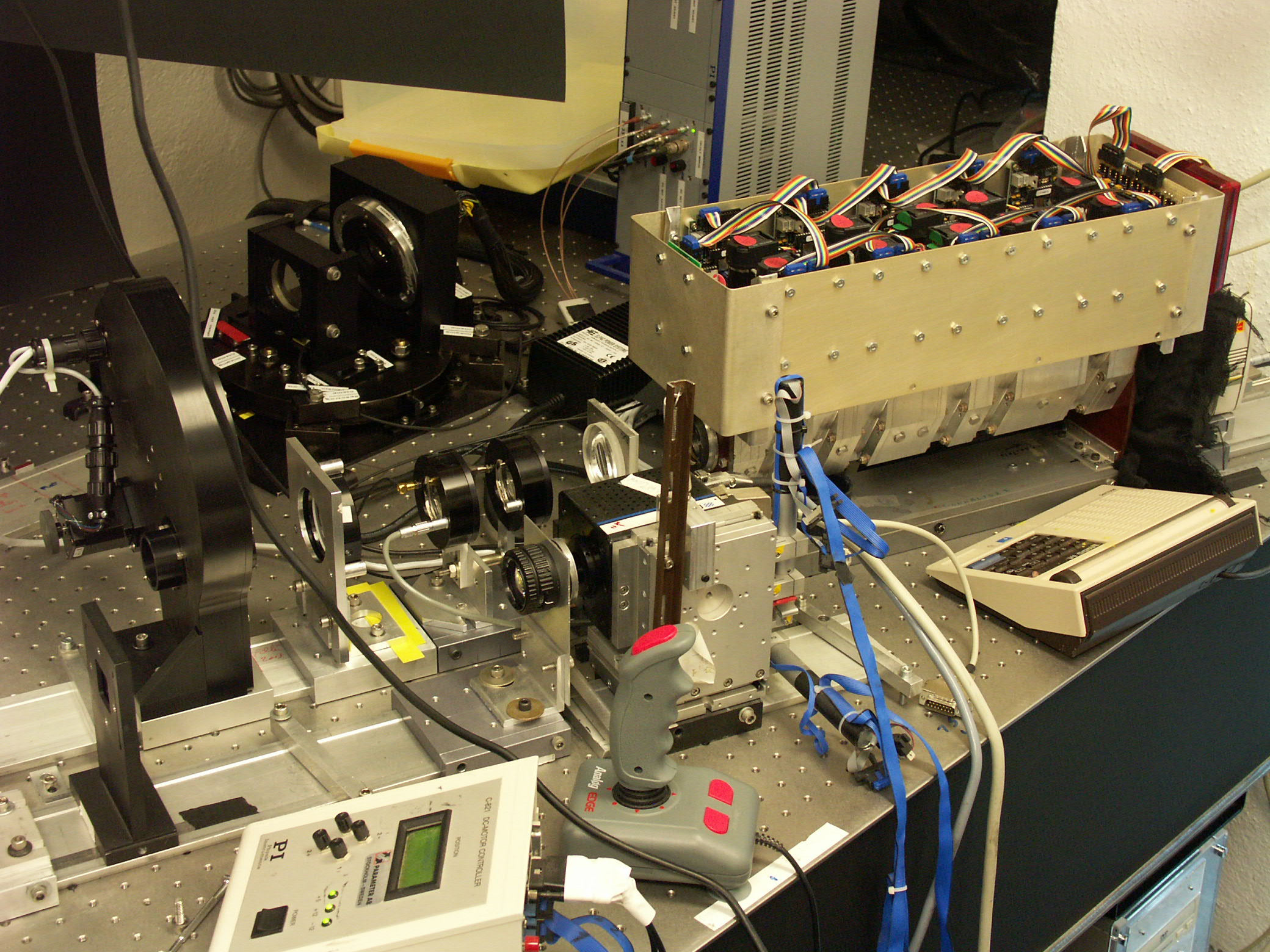
Fig. 1.1 The SOUP Filter installed at the SST. The light enters
from left. The blocking filterwheel (black, far left) precedes the collimator
lens, the LCVR stages, the camera lens, and the Lyot filter unit. The SST
Correlation Tracker is in the foreground.
2. Control
Unit
The control system is mounted above the Lyot Filter elements. This includes a motor control board for
each motor, a serial port converter board, a thermistor amplifier board, and a
Labjack data acquisition device.
The motor control boards are all daisy chained together starting with
the serial port converter (If you need to disconnect any of these wires, be
sure that the arrows on each connector/receptacle match up and connections
follow the figure below). External
connections to the control unit include the power supply input, a USB cable to
the Labjack, and a serial cable to the serial converter board. This control unit (new in 2004)
replaces the previous model, which featured a filter superstructure of motors
and wiring in addition to a separate rack-mount electronics box and power
supply.
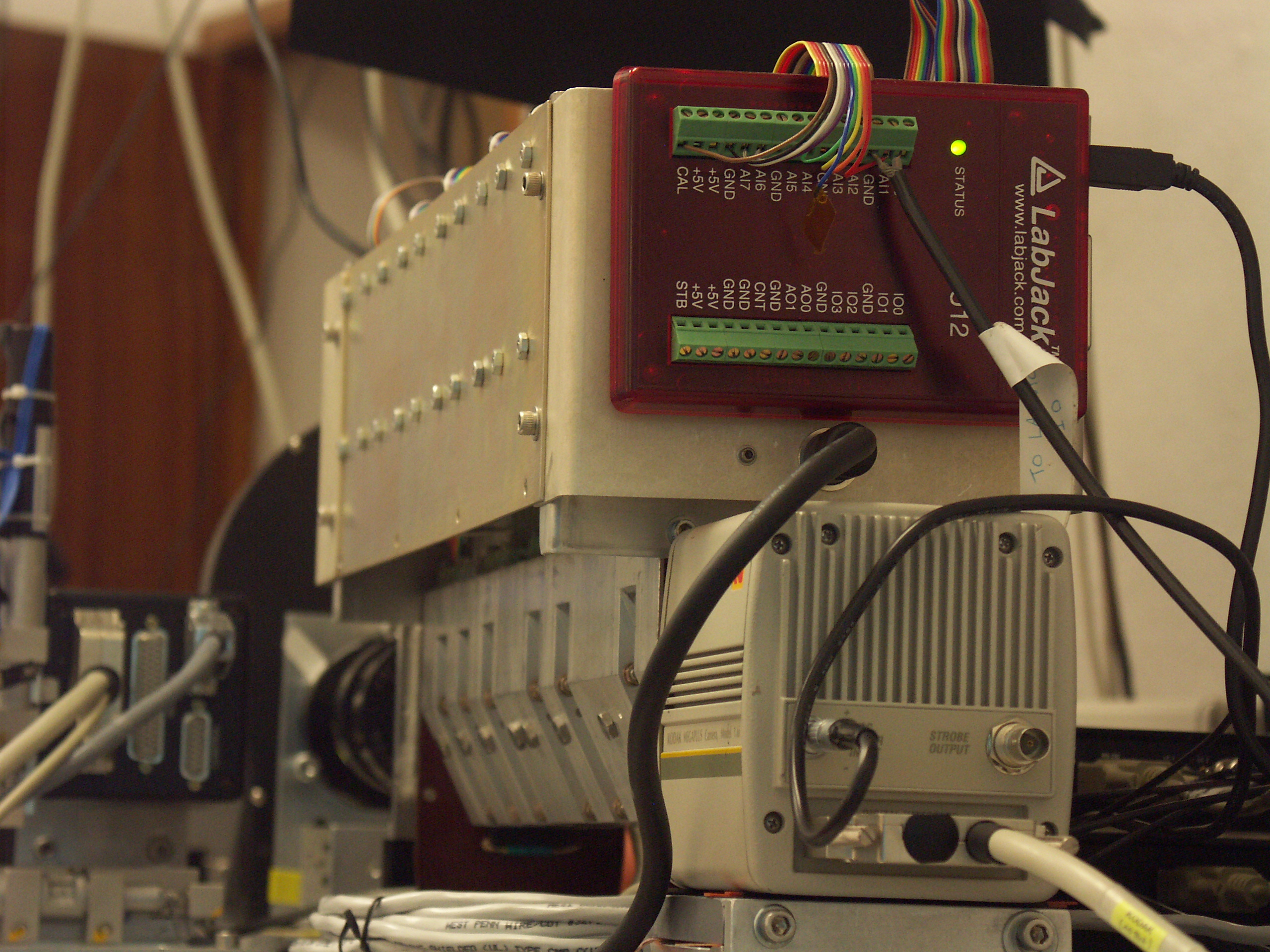
Fig. 1.3 Rear view of the SOUP Filter. The labjack unit with thermistor connection ribbon cable and photometer coaxial cable connected is visible above the black motor power cord. A Megaplus 1.6 camera is in place at the exit of the filter.
3. Main
Power Supply
Power is supplied to the filter assembly through a desktop power supply that
plugs into an end of the control box just below the Labjack. This power supply has a maximum power
of 48W, and is rated to accept both US and European AC inputs, but will need a
plug adaptor to accept non-US wall sockets. A pinout description is below.
|
|
Pin 1 |
2 |
3 |
4 |
5 |
|
COM |
COM |
+5 V 3.0 A |
-12 V 0.5 A |
+12 V 2.5 A |
4. Control
Computer
IBM laptop PC next to the Adaptive Optics terminal on the desk in the observing
room. The laptop connects to
peripherals through a USB port splitter and 3 USB-to-Serial converter
cables. On the USB port splitter,
connections are as follows:
|
Port 1: USB to Labjack |
Port 2: Serial to Motors |
|
Port 3: Serial to Meadowlark LCVR controller box |
Port 4: Serial to Filterwheel controller box |
In addition, the COM1 port on the back of the computer connects to the SOUP camera computer (currently royac19) via an RS-232 serial cable (null modem wiring).

Fig. 1.4 The SOUP Control Computer.
5. Photometer
System
This consists of the photometer head on the optical bench next to the end of
the TF Optical Assembly and the readout unit on top of the Adaptive Optics PC
beneath the optical table. BNC
output A from the readout unit connects to the Labjack analog input AI0 (center
wire) and GND (shielding) when the photometer is in use.
In normal use, the photometer is no longer used - line scans are now done using the science camera. See Section 4 for details.
6. 110-Volt
Transformer
Mounted under the table in the spectrograph room. This requires a particular
polarity of the 220V 50Hz European power for input. The correct polarity is
indicated by the plug with orange LEDs. IMPORTANT: if two LEDs are lit
then the input polarity is wrong and the Power Supply and other equipment MUST
NOT BE TURNED ON.
2. Connection Diagram
Below is a connection diagram of the current (summer 2004) SOUP filter arrangement. Light travels from right to left. The LCVR stages should normally be installed behind the blocking filterwheel. Image transfer optics (lenses) are not shown.
Click on the image for a (very much) larger image.

3. Start-Up Procedure
1. Boot up the TF PC if it isn’t already up.
There is no password protection on this computer, THEREFORE DO NOT PUT IT ON
THE NETWORK – it is vulnerable to takeover by login sniffers.
2. Plug in the power supply cable to the filter rear faceplate.
There is no power switch for the new SOUP motors. During normal operations, it is recommended to leave the motor power on at all times.
3. Turn on the D3040 LCVR
controller box .
This is a slim black box marked "Meadowlark D3040". It is currently on top of the filterwheel control box on the optical table behind the Lyot filter. The switch is on the front of the unit.
4. Double click on the
"Soup Filter" icon on the desktop to start the control code.
The icon may be behind other windows on the desktop. A DOS window will open and
various initialization tests be performed. When finished a main menu should
appear as shown in Fig. 3.1.
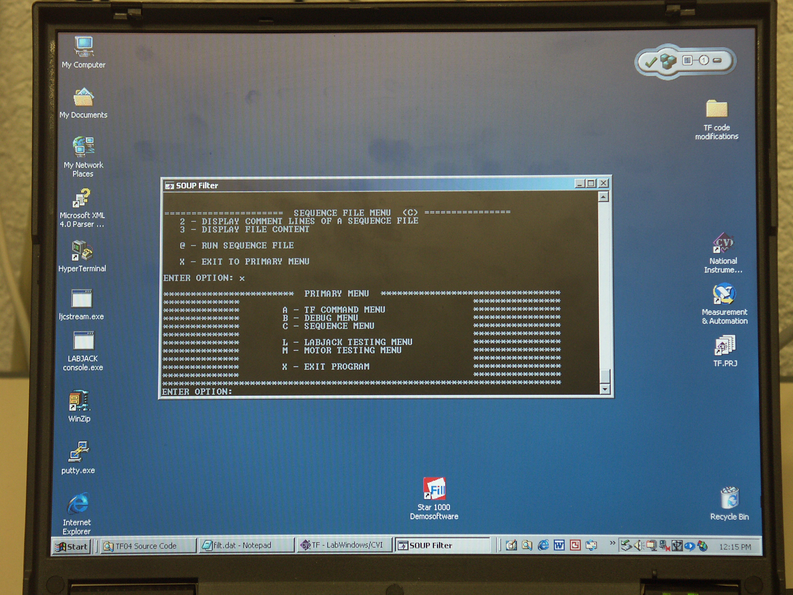
Fig. 3.1 The SOUP Filter "Primary Menu" (lower half of screen). This menu appears after a successful startup of the tf.exe program.
4. TF Calibration: Line Selection and Line Scans
The line center tunings for all available spectral lines have been calibrated in the laboratory and stored in a file called "filt.dat" in the TF source code directory. However the line center wavelength when observed on the Sun changes with disk position of the intended observing target due to solar rotational Doppler effect (convective blue shift and gravitational red shift also effect . Therefore before the SOUP filter can be used in observing mode, the line center wavelength of each spectral line in the observing sequence to be run must be calibrated at the location on the disk of the intended target.
There are two ways to measure line center positions: the preferred method uses the science camera in a special integration mode; an older method uses the external photometer. Both methods are described here, but we emphasize that the photometer method produces much noisier line profiles that often make it difficult to accurately find the line center. The disadvantage of the camera method is that the camera computer cannot automatically relay the line center wavelength back to the SOUP computer and so it requires more manual steps to accomplish the calibration.
1. Science Camera Line
Calibration.
In this mode, the science camera acts as an integrating detector to measure an average intensity for each spectral line position in a scan. It has the major advantage that you do not move the camera from its focused position and you therefore do not have to redo your flat fields every time you do a line scan (as with the photometer method).
A.
Point the telescope to your intended observing target.
If necessary, slightly off-point so that there are no sunspots in the view field.
B. Start the megaplus camera. Type "tcl/run_ccd.tcl m16-soup" from the /home/obs/cameras
directory.
Ensure that the m16-soup config file has the SOUP_TTY line defined. Call Pete Dettori if you're unsure about this step.
C.
In the Megaplus Camera Control GUI, set the mode to
"SOUP Calibrate" mode.
Set the reference exposure to a level which will correspond to the "1.0" relative exposures in your sequence file.
You may have to iterate this a bit using manual tuning of the filter (see Section 7) or by stopping and restarting this line scan procedure.
Set the number of repeats to 0.
Set the number of frames to measure to an even number (to take into account the even-odd shutter asymmetry).
2 is a good enough value.
Set the frame selection box to a large size (1000x1000 is good).
This is the area on the sensor over which the camera averages the intensity in order to calculate the line depth.
Press the START button.
The graphic window should open but remain white; a message saying "waiting for SOUP filter to give goahead" should appear in the text window.
D.
From the SOUP Filter Primary Menu
Select Option A: TF Command
Menu.
Select menu option "M": Manual line scan.
Set the filter in Wide or Narrow mode as prompted by the program.
Select the line you wish to calibrate.
The available lines are listed in Appendix A. Choose the spectral line number from the laboratory-calibrated line list which are numbered from 20 to31. For example, the H-alpha lab setting is Line 29, the FeI 6302.5Å lab setting is line 28.
Set the starting wavelength offset for the scan. This is usually –300 mÅ for the narrower Fe lines, and –1500 mÅ for H-alpha.
Set the ending wavelength offset for the scan. Usually the positive value of the starting offset for a symmetric scan.
Select the step size for the scan. A value of 20mÅ is usually sufficient to give a fine gradation in the line intensity.
Enter 'y' to scan in coordination with the camera.
Hit ENTER to send the go-ahead signal to the camera and start the scan.
The filter will tune to the starting offset from the nominal line center position and the camera will take N images. The camera computer then averages the intensity within the frame selection box of these N images and writes the offset in mÅ and the average intensity to a file in the /home/obs/cameras directory after the line scan is done. The camera then signals the SOUP computer to tune to the next wavelength position and the cycle repeats until the ending line offset is reached.
D. Plot the results of the line scan using ANA.
Go to the science camera computer. In the /home/obs/cameras directory type 'ana soupcal' at a shell prompt. This will plot the latest calibration file in the directory (the files for each scan are date/time stamped in their filenames; see top of Fig. 4.1 for an example filename ).
Examine the plot: it should look like a wide spectral absorption feature on an uneven continuum background. If you don't see any semblence of a spectral absorption line, check the exposure level and offsets and start over.
In the plot window, Select left-most (blue) wavelength over which to fit the resulting line profile by clicking with the mouse at the approximate offset position.
Select the right-most (red) wavelength for the fit.
The program will then fit a gaussian profile to the range selected and report the minimum value. This value should not be much different than the absolute minimum of the plot (reported on the ANA text window). A successful line scan is shown in Fig. 4.1.
Record this offset value for the next step.
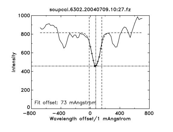
Fig. 4.1. A wide scan of the 6302.5Å from –700 to +700 mÅ with 20 mÅ steps.
The calculated offset is +73mÅ. The two satellite lines are the telluric O2 absorption lines.
E. Store the recorded line offset value in the filt.dat
file.
From the TF Command menu, type "L" to select "Set filter to a line". Set the filter to the laboratory reference wavelength. Use wide or narrow mode – whichever matches the mode used in the scan.
Once the filter is finished tuning to the reference wavelength, type "O" to "Offset the filter from here". Enter the offset you recorded from the line scan plot (in mÅ). Hit ENTER to accept element 8 as the last element tuned in the filter.
Type "S" to store the current motor and temperature values corresponding to the measured line center wavelength in the filt.dat file.
Enter the line number to store the new line position to. This number is the number of the lab line you scanned modulo 20. e.g. if you scanned the H-alpha laboratory setting (line 29) then you would enter "9" for the line number to which the current settings will be stored.
Type "9" to update all 9 elements of the SOUP filter to the new settings.
Type "Y" to acknowledge that you are updating a sequence line and you are sure that you want to do this. Check one more time that the number you entered above corresponds to the correct wavelength.
Enter a "name" for the new settings. This is usually the wavelength in Å and a short descriptor such as "FeI" or "H-alpha".
Type "Y" to accept the new name.
The new motor positions and temperatures for one spectral line are now stored in the filt.dat file. The entry is date stamped so if you're unsure if the filt.dat file has been properly updated, you can look at it (it is a text file) to be sure.
You are now ready to run an observing sequence.
2. Photometer Line Calibration.
TF line calibration consists of placing the photometer behind the filter and recording light levels as the filter is tuned through a specified range around a given line. A plotting program then shows you the resulting line profile and allows to you move the line bisector to the line center position corresponding to a given shift. This shifted position is then saved to the filt.dat file..
A. Slide the camera away from the filter.
There should be about 25cm of space between the camera and the TF.
B. Place the photometer head against the exit window of
the TF.
Wrap the black cloth around the gap to avoid scattered light into the
photometer.
C. Switch on the photometer readout below the optical bench.
D. In Menu A: TF Control, Select “I - Set filter to a line and start scan.”
Set the filter to Wide mode for H-alpha (in general) and Narrow for magnetogram or Dopplergram observations.
Choose the spectral line from the laboratory-calibrated line
list.
These are lines numbered 20-29. For example, the H-alpha lab setting is Line
29. If you choose Line 9 (the operational H-alpha setting) the filter will tune
to the previously shifted line position which may not be appropriate for your
particular disk position.
Select the range over which the scan will tune.
For narrow lines like FeI 6302 and NiI 6768 -300 to +300mA is usually sufficient.
For wide lines like H-alpha this is usually -1500 to +1500 mA.
When the filter is tuned it will say “Check setup....”
At this point, hit the “AUTO SCALE” button on the photometer to maximize the
gain. Once the photometer readout is stable and non-zero (usually in the 10s of
nano-Watts). Hit the AUTO SCALE button again to take the photometer out of
auto-scaling mode!
If something is wrong (no signal, wrong line, filter got the wrong blocker...)
Hit “A” to abort the line scan and start over.
Point to the observing target on the Solar disk if you’re not already there.
Hit RETURN to start the line scan.
This takes about 2-4 minutes depending on the width of the scan range selected
above. When finished, a GUI plot window will appear with the data plotted.
Locate the line center offset.
Using the cursor, click on the position of the line center. Alternatively, use
the left- or right-arrow keys to move the cursor along the plot point-by-point
until it is at your chosen line center position.
Press ‘Quit-Save cursor location’ to exit the plotting
program and save the line in the filt.dat file.
You should return to Windows mode and the TF application window should have
output indicating that the line was saved in “Line 8”, for example, if you have
just finished scanning Line 28. Lines are only saved modulo 20 in order to
avoid overwriting the laboratory calibrations.
Repeat step D on every line that you intend to observe.
Remember to save each line bisector before exiting.
E. Remove the photometer and replace the camera behind
the filter.
Perform new flatfields since you have moved the camera relative to any
previous flats.
You are now ready to run an observing sequence.
5. Running Observing Sequences
Observing sequences for the TF are contained in text files in the D:\SOUP\Sequences folder. They are suffixed by “.seq”. Each file contains one text line for each spectral line position and/or polarization that will be observed. Comments are denoted by semi-colons “;”. Post-fixed comments are allowed on any line – everything after the semicolon will be ignored by the program.
Basic observations with the TF involve reading the chosen SEQ file and repeating the individual entries in the order they are written in the file in coordination with the frame selection operation of the camera. The number of times the sequence repeats can be chosen by the user.
The structure of a sequence is exemplified by the following simple sequence called HAMAG.SEQ. This sequence takes images at each of 4 positions in the H-alpha line followed by three images in the Fe I 6302.50A magnetic line. Comments are preceded by semi-colons and can occur on lines by themselves or after the sequence information. Spacing between the items does not matter.
|
|
;Fast Halpha w/ 6302 magnetic mode |
|
|
|
Examining the first non-comment line, “fpic” is the designation for a filtergram picture - it’s used for all lines. Some older sequences may have "vpic" here – ignore this difference.
”9” is the line number corresponding to the entry in the filt.dat file
and (hopefully) matching the line numbers in Appendix
A, in this case H-alpha.
”-700” is the offset from line center in milliAngstroms.
”1” indicates that the filter is in wideband mode, used for wide lines such as
H-alpha. A “0” in this position indicates narrow bandpass mode, used for
magnetic and Doppler lines.
”0” in the 5th column indicates no polarization state is set in the
LCVRs. LCP and RCP indicate left- and right-circularly polarized states,
respectively.
”0.8” is the relative exposure factor for this line setting. If the nominal
camera exposure in the control GUI is X msec, this image will be taken
with an exposure of 0.8X msec.
"1.8" is the delay (in seconds) that the program will wait for the filter to tune before giving the go-ahead to the science camera.
To run a particular sequence file do the following:
From the Primary Menu press ‘C’ to get to the sequence menu.
Type ‘@’ to prompt for the sequence filename you wish to use.
Type the filename of the sequence you wish to use.
The program will echo the contents of the sequence file. Hit ENTER to continue.
Enter the number of loops through the sequence file and
the delay (in seconds) before start
DO NOT HIT RETURN!
The number of loops should be set to 1000 or some high number for long periods
of uninterrupted operation. The delay is typically 0 since this function is now
handled by the delay values written in the sequence file.
Start the Megaplus camera in Frame Selection Mode.
Type “tcl/run_ccd.tcl m16-soup” from the /home/obs/cameras directory to start
the megaplus program which communicates via serial line with the TF computer.
Once you have determined you frame selection and exposure parameters, hit the
START buttton. It should open the display window but not start taking
frames. A message in the text output window should say “Waiting for SOUP filter
to give goahead.”
Return to the SOUP computer and hit RETURN.
The filter will tune to the first setting in the sequence file and the camera
should begin taking frames for frame selection. The TF program will say
“Waiting for a T from the camera computer...” while frame selection is in
process. At the conclusion of the frame selection period, the filter should
proceed to the next setting in the sequence file.
Adjust the base exposure of the camera.
The base exposure is the exposure time in the megaplus GUI. This corresponds to
a relative exposure factor of 1.0 in the sequence file. Adjust the base
exposure to give the desired signal level for the 1.0-factor images. If the
other images in the sequence with relative exposures less than or greater than
1.0 are under- or over-exposed, you should stop the sequence and edit the
sequence file to correct the relative exposure factors. See Editing Observing
Sequences for instructions on editing files.
To STOP the sequence:
A. Hit ‘Q’ on the TF computer keyboard OR ...
B. Press STOP in the camera GUI. Then hit ‘Q’ on the TF keyboard.
To exit to the SOUP Primary Menu, type ‘x’ and hit RETURN.
6. Editing Observing Sequences
Observing sequence files are simple text files that can be edited with the editor of your choice. Double-clicking on a .SEQ file will open it in WordPad, a Microsoft product that tries to make you save it in MSWord format. Be sure to save the file in ‘Text Document’ format, not in ‘MS Word 6.0’ format. Other than that, it’s the simplest way to edit the files.
Make sure that you do not have any characters (including spaces) on the line following the last line of the sequence file. If so, you will get an error in the Copycheck() function of the Sequence running routine.
Also, make sure you get rid of the default ".txt" suffix that may be added by the editor. The SOUP program only recognizes files with the ".seq" suffix.
7. Running in a Single Line Position
If you wish to run continuously in a single line position and a single polarization, you don’t need to run a sequence file. In this case, you simply set the filter to a (previously calibrated) line center, offset from the line center by the desired amount, and set the polarizer wheel to the desired polarization setting. This is detailed in the steps below.
1. From the Main Menu, select ‘A’ TF Control Menu.
2. Select ‘L’ Set Filter to a line.
A. Note the status of the “Wide/Narrow” setting of the
filter.
If you want to change the mode, type ‘S’ and then ‘N’ for narrow or ‘W’ for
wide mode.
B. Enter the line number of the desired spectral line and
offset from line center
Line Number: see the Appendix
A.1: Line List for the full list of available spectral lines. Lines
numbered 1-12 are the solar-calibrated line tunings; lines numbered 20-32 are
laboratory settings. For observing targets on the Sun, you should choose one of
the solar-calibrated lines (see the instructions on TF Calibration for instructions
on line position calibration).
Offset from line center: entered in milliAngstroms; negative values are blue offsets, positive are red.
Cold or warm start: this refers to the ability of the SOUP filter to correct tuning motor positions based on a HeNe laser alignment procedure. It is essentially an obsolete procedure: enter ‘0’ for cold starts of all lines.
The filter should set the appropriate blocker and then tune the motors to the requested line position. Hit any key to return the to the TF Control menu.
3.
Select ‘W’ “Where am I now?”
This prints the wavelength that the filter believes itself to be set to. It is
NOT a measurement; it is only a tabulation of the requested line position and
offsets; it should only be used as a rough check on the approximate wavelength
setting of the filter.
4. Select
‘J’ to change the polarizer to the desired position.
Enter the polarizer type in uppercase letters. See Appendix A.1: Polarizers for the
list of available polarizers.
You are now ready to run the camera in Frame Selection mode. For this, you need to run a megaplus program other than m16-soup since you want the camera to operate without waiting for the filter to send serial-line signals. Contact Pete Dettori (dettori@astro.su.se) for instructions on using different megaplus programs.
1. Flat and Dark Field Images
You need flat field and dark current images for each line position and polarization that you took data images in.
Flat fields and dark images are run in the same way that sequences are run. The easiest thing to do is to run both a flat and a dark series for each sequence that you ran during the observing period. The basic steps are as follows:
1. Set
the telescope to FlatField mode (for flats) or block the light (for darks).
2. Set the camera mode to “Flats” or “Darks”. Note: As of 8-July-2004 the Darks mode was not communicating with the SOUP control computer. The solution is to run the camera in flat field mode and note down the file numbers in your log as being dark frames.
3. Set the Repeat count in the camera GUI to 0.
4. Set the baseline exposure to match the exposure that you were running the given sequence at.
5. Set the number of frames to 50 or 100 or however many frames you want averaged to make your flat or dark image.
6. Hit
the START button.
The display window should open and a message saying “Waiting for SOUP filter to
give goahead” should be sent to the terminal window.
7. Go
to the SOUP computer and run the appropriate sequence.
For the number of repeats, type in the number of flats or darks that you want
to have for each wavelength/polarity position. This is a minimum of 2 and
usually less than 5.
2. Shut-Down Procedure
1. Exit to the Main Menu by typing ‘X’ in any of the sub-menus.
2. From the Main Menu type ‘X’ and then ‘y’ to accept an exit from the program.
3. Turn off the TF Power Supply with the toggle switch on the front panel.
4. Turn off the Photometer.
10. Error Handling
No other significant errors have been noticed during the 2004 observing season.
Appendices
A. Spectral Line List
Currently
the only lines available are the following:
Line Number
|
Wavelength
Å
|
FWHM, Narrow
mÅ
|
FWHM, wide
mÅ
|
Comments
|
21
|
6328.17
|
75
|
118
|
Laser line and solar continuum
|
24
|
5576.10
|
56
|
92
|
Fe I g = 0 Dopplergram line
|
28
|
6302.50
|
72
|
118
|
Fe I g = 2.5 magnetogram line
|
29
|
6562.80
|
78
|
128
|
H-alpha
|
31
|
6301.50
|
72
|
118
|
Fe I g = 1.5 magnetogram line
|
The Fe I magnetogram lines use the
same blocker.
B. TF Menu Reference
************************ PRIMARY MENU
*********************************
**************
****************
************** A - TF COMMAND MENU
****************
************** B - DEBUG MENU
****************
************** C - SEQUENCE MENU ****************
**************
****************
************** L - LABJACK TESTING
MENU
****************
************** M - MOTOR TESTING
MENU
****************
**************
****************
************** X - EXIT PROGRAM
****************
**************
****************
*************************************************************************
======================== TF COMMAND MENU (A)
============================
A - ALIGN FILTER W/ LASER
L - SET FILTER TO A LINE
B - SET WIDE OR NARROW
M - MANUAL LINE SCAN
D - DISPLAY MOTORS ELEMENTS TEMPS O - OFFSET FILTER FROM HERE
E - EXPERIMENT LOG FILE CONTROL P - POLARITY CHECK
H - HOME ALL MOTORS
R - RUN ALL MOTORS FOR WARMUP
I - PERFORM LINE SCAN
S - STORE LINE PARAMS TO FILT.DAT
J - SET POLARIZER
W - WHERE AM I NOW?
K - SET BLOCKER
V - REPORT BLOCKER POSITION
X - EXIT TO PRIMARY MENU
Z - DISPLAY MENU
========================================================================
======================= DEBUG MENU (B)
============================
A - DISPLAY MOTOR POSITIONS L - SET
FILTER TO A LINE
B - CHECK FOR MOTOR HOME
M - TUNE FOR MAXIMUM
C - HOME ONE OR ALL MOTORS P -
DISPLAY LCVR VOLTAGES
D - DISPLAY MOTORS ELEMENTS TEMPS
E - SET POLARIZER
S - STEP ONE MOTOR
F - SET BLOCKER
T - TUNE ELEMENT
W - CHANGE MOTOR 9 WIDE
U - MULTI-STEP TO POS x
X - EXIT
Z - DISPLAY MENU
====================================================================
====================== SEQUENCE FILE MENU
(C) ================
2 - DISPLAY COMMENT LINES OF A SEQUENCE FILE
3 - DISPLAY FILE CONTENT
@ - RUN SEQUENCE FILE
X - EXIT TO PRIMARY MENU
=================================================================
======================= MOTOR TEST MENU
=========================
1 - HOME one motor to ENCODER HOME, no position zero
2 - HOME all motors to ENCODER home, no position zero
3 - DEFINE current position for Motor X as zero
4 - MOVE motor X to PIC-position Y
5 - STEP one motor by 1/48 rev in CW or CCW direction
6 - STEP one motor by N steps in CW or CCW direction
7 - MOVE motor X to SOUP Y by steps
8 - MOVE all motors to position array
9 - HOME one motor to SOUP home position
A - HOME all motors to SOUP home position
B - STARTUP homing sequence for all motors
C - SEND one motor to SET_SCREW ACCESS position
D - SEND all motors to SET_SCREW ACCESS position
E - MOVE one motor to SOUP position Y
F - REPORT motor positions
X - EXIT TO PRIMARY MENU
======================================================================
=================
LABJACK DEBUG MENU (F)
===================
1 - THERMISTOR CALIBRATION PROCEDURE
2 - LOAD readtemps[] ARRAY
3 - READ PHOTOMETER
4 - PLOTTING ROUTINE TEST
X - EXIT TO PRIMARY MENU
==============================================================
C. Blocking Filter Wheel Positions
Blocker Number
|
Wavelength
Region
Å
|
0
|
6328
|
1
|
6563
|
2
|
6302
|
3
|
5576
|
4
|
Open
|
5
|
Open
|